The criptic test suite
This page summarizes how to run the test suite and examine results (Testing workflow), and briefly describes each problem (Available test problems). It also provides a guide to Writing new tests.
Testing workflow
Testing involves three stages: Compiling one or more test problems, Running them, and Analyzing the results by comparing to known solutions.
Compiling
Criptic test problems are located in the Src/Prob/Test directory. They can be compiled individually, as for any criptic problem, by doing:
make PROB=Test/NAME_OF_TEST
in the main criptic directory. It is also possible to compile all the tests at once, by doing:
make tests
in the main criptic directory. To test with MPI or OpenMP disabled, you can use the same flags as with any other make command – see Building criptic.
Running
Each test problem comes with a parameter file called criptic.in, located in the same directory as the problem setup files.
Individual tests can run as with any other criptic problem: cd into the test problem directory, and run the code by doing:
criptic criptic.in
or:
mpirun -np NUM_PROCESSES criptic criptic.in
to run on multiple MPI ranks.
Criptic also provides a python script, runtests.py, in the Src/Prob/Test/ directory, which can run and then analyze all of test problems or a subset of them. To use this script, simply do:
python Src/Prob/Test/runtests.py
from the main criptic directory. To run only some of the tests, do:
python Src/Prob/Test/runtests.py --tests [TEST1 TEST2 ...]
where TEST1 and so forth are the names of the test problems to run. By default the output produced by running each of the individual tests will be redirected to an output file test.log in the directory containing the test, though this can be overridden (and the output printed to the screen) via the option verbose.
Caution: running the entire test suite is likely to require several hours on a typical desktop or laptop.
Analyzing
Each test problem comes with an analysis script, called analyze.py, located in the same Src/Prob/Test subdirectory as the problem setup and parameter files. After running an individual test, you can check the results against the reference solution by doing:
python analyze.py
from the same directory where the test was run. By default, the analysis script will just return a result of PASS or FAIL, and will produce one or more diagnostic plots, with names of the form TESTNAME1.pdf, TESTNAME2.pdf, etc. These generally show a comparison of the test result against an exact solution; the figures produced generally match those shown in the test problems presented in the criptic method paper. If you want slightly more information, e.g., the exact L1 errors produced by the test, you can do:
python analyze.py --verbose
If you are using the runtests.py script (see Compiling), there is no need to run the analysis separately. This script will automatically run the analysis on each of the test problems it executes and report the result. If all tests are successful, the output of runtests.py will be:
Running test AnisoDiff...
    PASS
Running test AnisoDiffLoss...
    PASS
Running test ElectronStreamLoss...
    PASS
Running test LoopDiff...
    PASS
Running test MomDiff...
    PASS
Running test NdenComp...
    PASS
Running test NonLinDiff...
    PASS
Running test PitchAngleDiff...
    PASS
Running test RadStream...
    PASS
Running test VarDiff...
    PASS
Available test problems
Here we list the available test problems:
Derivations of the exact solutions to which these tests compare, and complete descriptions of the problem setup and motivation, are included in the criptic method paper.
AnisoDiff
This test evaluates criptic’s ability to simulate anisotropic diffusion with a diffusion coefficient that depends on cosmic ray energy. Three point sources with luminosity \(L = 10^{38}\) erg s-1, injecting cosmic ray protons with kinetic energyes of 1, 10, and 100 GeV, are placed at the origin of an infinite, open domain. The background magnetic field is uniform in the x direction. The perpendicular and parallel diffusion coefficients are given by
All losses are disabled. Here we show typical output of a successful test. The top panel shows energy density versus normalized radius for each of the three cosmic ray energies, and the bottom shows a projection of the cosmic ray energy density for one of the energies.


AnisoDiffLoss
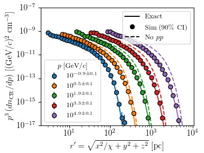
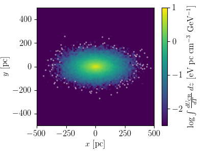
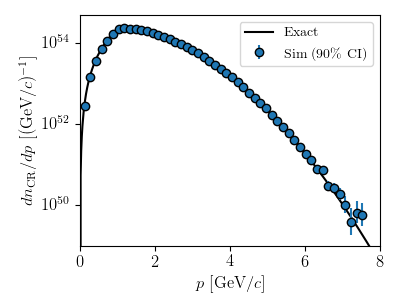
This test uses the same basic setup as AnisoDiff, but instead of three sources injecting cosmic rays at discrete energies, there is a single source that injects cosmic rays with a momentum distribution \(dn/dp\propto p^{-2.2}\) over a momentum range from 0.1 - 105 GeV/c. The background gas density is \(\rho = 2.35\times 10^{-21}\) g cm-3, and nuclear inelastic losses are enabled; all other losses remain disabled, and secondary particle production is also disabled. The test compares the energy density as a function of radius and cosmic ray energy to the exact solution, including the effects of losses.
The figures below show typical outcomes. The top panel shows the cosmic ray number density per unit momentum (scaled by \(p^3\) to make the different momentum bins easier to compare) as a function of radius, compared to the exact result. The dashed lines labelled “No pp” show the exact result without losses for comparison. The bottom panel shows a projection plot of the specific energy density.
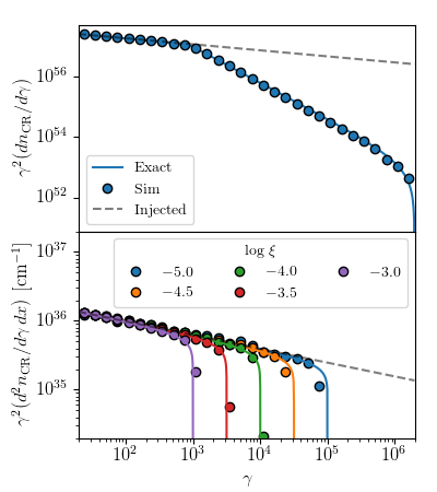
ElectronStreamLoss
In this test a point source of cosmic ray electrons with luminosity \(L = 10^{38}\) erg s-1 is placed at the origin; it injects cosmic rays with a momentum distribution \(dn/dp \propto p^{-2.2}\) from 0.01 - 1000 GeV/c. The cosmic rays stream along the magnetic field, which is oriented in the x direction, at a constant speed of 100 km s-1. The region is suffused with a background radiation field and magnetic field, both of which have energy densities of 50 eV cm-3; the radiation field has a blackbody temperature low enough that all electrons are in the Thomson limit. As the electrons travel down the field, they lose energy to inverse Compton and synchrotron radiation. All other loss mechanisms are disabled. This tests the code’s ability to calculate these loss rates, and produce the correct electron energy spectrum.
The figures below show typical outcomes of a successful test. The top panel shows the cosmic ray momentum distribution (with momentum expressed in terms of the Lorentz factor \(\gamma\)) integrated over all space, and the bottom panel shows the momentum distribution evaluated at five different distances from the source, with distance expressed in terms of the dimensionless position \(\xi\).
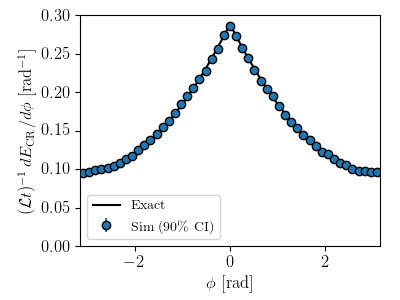
LoopDiff
In this test the magnetic field is arranged in a circular loop. A point source of cosmic ray protons with luminosity \(L = 10^{38}\) erg s-1 is placed along with loop, at a radius of 1 pc from the center. Cosmic rays travel by diffusing, wiht a diffusion coefficient \(k_\parallel = 10^{28}\) cm2 s-1 along the field and zero perpendicular to the field. In addition, the source and the magnetic field also undergo simple harmonic oscillation in the plane of the field loop. This problem tests criptic’s ability to follow cosmic rays correctly as they diffuse along a bent, accelerating field line. All losses are disabled for this test.
The figure below shows the results of a successful test. The plot shows the density of cosmic rays per unit angle along the field loop.
MomDiff
This test evaluates criptic’s ability to follow diffusion in momentum space. A source of cosmic ray protons with luminosity \(L = 10^{38}\) erg s-1 injects cosmic rays with initial momentum \(p_0 = 1\) GeV/c. These do not move in space or suffer losses, but diffuse in momentum with a diffusion coefficient \(k_\mathrm{PP} = p_0^2 / t_\mathrm{diff}\) with \(t_\mathrm{diff} = 1\) Myr. The protons then diffuse in momentum space, and the test compares the momentum distribution after some time to the exact solution.
The figure below shows the outcome of a successful test, comparing criptic’s calculated momentum distribution to the exact solution.
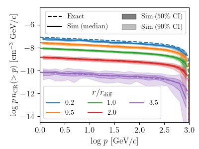
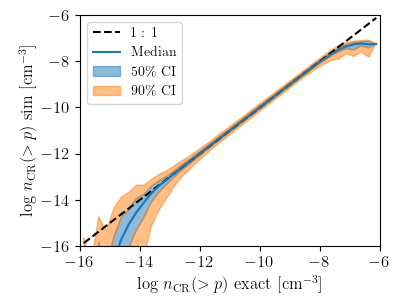
NdenComp
This problem uses the same setup as AnisoDiff – a point source at the center of a region of uniform magnetic field, with no losses or streaming, just diffusion – but with a point source that injects protons with a momentum distribution \(dn/dp \propto p^{-2.2}\). In this test the code calculates the cumulative number density of cosmic rays as a function of position and momentum, and compares to the exact solution. This tests the kernel density estimation method for reconstructing field quantities.
The figures below show the outcome of a successful test. The top panel shows cumulative cosmic ray number density as a function of momentum at several radial locations, and the bottom shows a packet-by-packet comparison of the exact and reconstructed cosmic ray number densities.
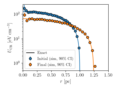
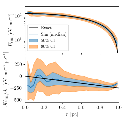
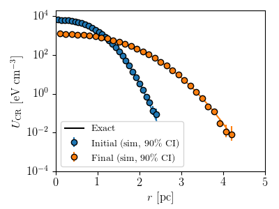
NonLinDiff
This test evaluate’s criptic’s ability to solve non-linear diffusion problems. It begins with a spherically-symmetric distribution of cosmic ray protons, whose density as a function of radius matches a similarity solution for non-linear diffusion, with an isotropic diffusion coefficient that varies with the cosmic ray energy density as \(k \propto U\). The test is to verify that the cosmic ray energy density continues to evolve following the similarity solution, and, in particular, that the outer edge of the distribution, where the energy density goes to exactly zero, expands matching the analytic result. Losses are off for this test.
The figures below show the results of a successful test. In the first panel, the blue points and line show the simulation state and similarity solution at the initial time, and the orange points and line show the simulation state and similarity solution at the final time. The second panel shows the criptic reconstruction of the cosmic ray energy density and its radial derivative at the initial time, as compared to the exact result.
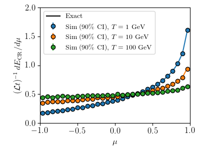
PitchAngleDiff
This test evaluate’s criptic’s pitch angle diffusion code. The test begins with three sources with equal luminosities, injecting monoenergetic cosmic ray protons with three different energies. The cosmic rays are all injected with pitch angle \(\mu = 1\). The cosmic rays scatter in pitch angle with a constant diffusion coefficient \(k_\mu \propto p^{1/2}\), where p is the CR momentum. The test checks that the pitch angle distribution of the CRs one diffusion time later matches the exact solution for spherical diffusion from a point source.
The figure below shows the results of a successful test. Solid lines show the analytic solution for the CR energy per unit pitch angle, which is different for each of the three CR kinetic energies \(T\) due to their different diffusion coefficients. Circles with error bars (which are mostly too small to see) show the median and 90% confidence interval for the numerical solution computed by criptic.
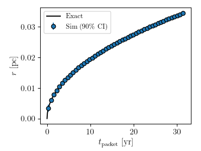
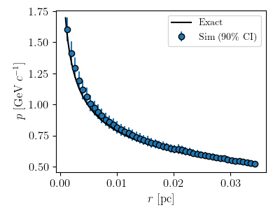
RadStream
This test evaluate’s criptic’s ability to handle problems in which cosmic rays stream in a direction opposite the cosmic ray pressure gradient, making the problem non-linear. A monoenergetic point source of cosmic rays is placed at the origin of a region where the magnetic field is a split monopole, so the field lines point radially outward. Since the cosmic ray pressure gradient is always pointing toward the origin, where the source is located, the cosmic rays should always stream radially outward. The propagation model is that the streaming speed is equal to the ion Alfvén speed, and the density and magnetic field strength vary with radius, so the streaming speed also varies with radius. This in turn means that the cosmic ray packets undergo adiabatic losses as they move outward. Thus in this problem there should be a one-to-one relationship between the time at which a cosmic ray packet was injected, its radial position, and its momentum. The test is to verfiy that criptic reproduces this relationship.
The figures below show the results of a successful test: the top panel shows raddius versus time, and the bottom shows momentum versus radius.
VarDiff
This test evaluates criptic’s ability to solve a problem with a non-constant diffusion coefficient. Cosmic ray transport is via isotropic diffusion, with a diffusion rate coefficient that is a powerlaw function of radius and time:
with \(r_0 = 10^{18}\) cm and \(t_0 = 10^8\) s. The problem then admits a similarity solution for the cosmic ray density as a function of radius and time. The test is to initialize the system to the similarity solutino at one time, then evolve it and verify that it matches the similarity solution at a later time. All losses are off.
The figure below shows a successful test result. The blue points and line show the initial simulation state and exact solution, respectively, and the orange points and line show the state at a later time.
Writing new tests
To write a new test, simply create a new subdirectory of Src/Prob/Tests containing your test. In that directory provide
A
Prob.cppproblem setup file (see Setting up a problem)A
criptic.infile containing the run-time parameters (see Parameter files)A python script called
analyze.pythat can be executed by typingpython analyze.pyat the command line, and printsPASSorFAILto report the result of analyzing the test. To be fully compatible with theruntests.pyscript, theanalyze.pyfile must accept the arguments--verboseand--testonly; the former causes more verbose output, and the latter suppresses production of the diagnostic figures.
Once these prerequisites are met, the test will be built by make tests and analyzed by runtests.py automatically.